We work with our partners very closely in order to incorporate their capital market views for returns, volatilities, and correlations for all asset classes in our ALM Studies. Where needed, we supplement our partners’ views with our own factor-based Capital Market Assumptions.
Overview of Predictive Factors
Empirical studies showed that stock and bond returns, interest rate term structures, and credit spreads can be predicted to some extent by certain Predictive Factors using predictive regressions that have the following general conceptual form:
return_{t+1}=\alpha+\beta_1 factor_{1t} +\beta_2 factor_{2t} +\beta_3 factor_{3t} +…+ \sigma_t \epsilon_t
- Observable, such as for example dividend yield or earnings yield.
- Non-observable, such as for example slope of the Treasury yield curve term structure.
- Expressed in a linear form as part of the predictive regression.
- Expressed in a non-linear form as part of the predictive regression.
- Asset class specific, i.e. some factors may be more applicable for only certain asset classes.
- Statistically significant coefficients \beta , i.e. they are not zero from the statistical stand point.
- High coefficients R^2 , i.e. they have good explanatory powers in relation to the appropriate asset class returns.
- Predictive Factors are based on current market data and reflect empirical evidence for the predictability of respective asset returns, yield curve term structures, and credit spreads.
- They can serve as State Variables fully integrated into multi-period dynamic stochastic portfolio optimizations.
- Predictive Factors can also be used as part of the factor-based analytics fully integrated into Liability Hedge Fixed Income Solutions.
- They facilitate building custom Glidepath Solutions, since only factors fully relevant to both assets and liabilities unique to a given pension plan are implemented.
Various Approaches to Capital Market Assumptions
The following table provides the overview of three methods used to create effective Capital Market Assumptions and compares these three methods based on certain metrics outlined on the left-hand side of the table.
Expected Return
\mu
Volatility
\sigma
Correlation
\rho
Randomly Simulated Returns
r
Return Distribution
Assumption
Fat Tails of
Return Distribution
Asymmetry of
Return Distribution
Fixed over time
\mu=const
Fixed over time
\sigma=const
Fixed over time
\rho=const
Returns simulated as
r = \mu+\sigma \epsilon
Usually
Normal Distribution.
Not implemented
Not implemented
Changes over time
\mu_{t+1}=\alpha+\beta \mu_t +\epsilon_{t+1}
Changes over time
\sigma_{t+1}=\alpha+\beta \sigma_t +\epsilon_{t+1}
Changes over time
\rho_{t+1}=\alpha+\beta \rho_t +\epsilon_{t+1}
Returns simulated as
r_{t+1} = \mu_t+\sigma_t \epsilon_t
Most distributions
implemented
Implemented
Implemented
Changes over time
\mu_{t+1}=f(\mu_t,factor_t)
Changes over time
\sigma_{t+1}=f(\sigma_t,factor_t)
Changes over time
\rho_{t+1}=f(\rho_t,factor_t)
Returns simulated as
r_{t+1} = \alpha+\beta factor_t+\epsilon_t
Most distributions
implemented
Implemented
Implemented
Simulated Returns Based on Predictive Factors
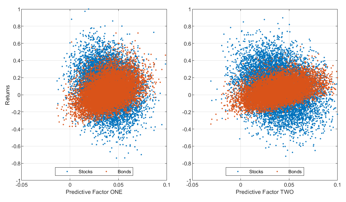
The following charts illustrate predictive relationship between two Factors and the respective returns of the Stock and Bond asset classes:
According to the following charts, Predictive Factor Two has stronger predictive properties than Predictive Factor One.
