Traditional ALM Studies for defined benefit pension plans represent multi-period stochastic simulations of Assets and Liabilities, where Investment Policy is typically one of many inputs. ALM Studies can also be run for several different Investment Policies and simulated ALM results can be used to compare these alternative asset allocations.
As such, a natural extension of traditional ALM Studies is to run them for numerous Investment Policies in order to choose one asset allocation that offers the best result and the most optimal outcome.
Therefore, ALM Studies can be used as part of numerical methods for solving complex and custom multi-period stochastic optimization investment problems for pension plans.
Portfolios Optimization: Stochastic vs Mean-Variance
Stochastic portfolio optimization is fundamentally different from traditional Mean-Variance type portfolio optimization as shown in the following table where a number of portfolio characteristics are compared:
Periods
Single-period optimization
Multi-period optimization
Risk Measure
Standard Deviation of asset returns
Downside level of Funded Status
Return Measure
Expectation of asset returns
Median level of Funded Status
Objective Function
Max Return for given Risk or Min Risk for given Return
Max Utility function, such as max Power Utility of Funded Status in 10 years
Generic or Plan Specific
Generic based on asset returns only
Pension plan specific
Pension Liability
Pension liability not reflected
Pension liability fully reflected
Inflows/Outflows
No Inflows/Outflows reflected
All Inflows/Outflows reflected
Customization
Limited customization available
Full customization available
Closed Form Solution
Closed form solution available
No closed form solution, numeric only
Computational Intensity
Low computational intensity
High computational intensity
Complexity
Low complexity
High complexity
Path Dependency
No path dependency reflected
Full path dependency reflected
ALM Study as Numerical Method for Stochastic Optimization
Stochastic portfolio optimization is very powerful and most relevant tool for pension plans since it completely reflects all pension plan specific liabilities, ERISA-PPA funding rules and cash inflows, benefit payment outflows, Funded Status and restrictions, plan specific de-risking goals, and many other custom objectives:
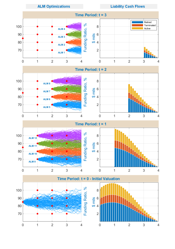
One such methodology is Backward Induction based Dynamic Optimization approach, which is used to solve recursive Bellman Equations based on the following conceptual steps as shown in the following chart:
We start at the beginning of the last period and run ALM Studies over the remaining one period for each level of Funding Ratios and Discount Rates from a grid, and for each ALM run find optimal allocation in the last period, by maximizing chosen expected Utility function (based on end Funded Status and all cash paid).
Then we move one step backward in time to beginning of the second to last period and run ALM Studies over the remaining two periods for each level of Funding Ratios and Discount Rates from a grid, and for each ALM run find optimal allocation in the second to last period, by maximizing chosen expected Utility function (based on end Funded Status and all cash paid), and by using optimal allocations in last period determined in prior step.
This process is repeated for each period moving backward in time until we reach valuation time zero.
The output of this process is Dynamic Asset Allocation, which represents optimal asset allocation at time zero as well as optimal asset allocations for each level of Funding Ratios and Discount Rates found in the grid for each future period used in the portfolio optimization.
